In the United States, sports are big business.  Roughly 154 million people watch live sports at least once a month.  And those numbers are expected to climb every year.

With the sports boom, cottage industries like fantasy sports, DFS, and prop-betting sites have given fans another reason to watch (and become more engaged).  These games allow shrewd viewers to earn big bucks by outsmarting other players (and sportsbooks) to win lucrative online contests.

The primary way that fantasy gamers gain an advantage is by using proprietary algorithms to project player performances.  Massaging player stats allows gamers to find obscure statistical gems they can leverage to win more contests.

Today, we’ll look at how you can accomplish this using Google Sheets.  We’ll prepare for a hypothetical fantasy draft by importing player statistics from a public website.  Then, we’ll use the power of functions to transform, manipulate, filter, and sort this data to our liking.

Publish Google Docs to your blog in 1-click

• ✅ Export in seconds (not hours)
• ✅ Less VAs, interns, employees
• ✅ Save 6-100+ hours/week

Check out Wordable now →

1.  Identify Your Target Data Source Online

Participants of fantasy football prize leagues know how important it is to evaluate and rank players before a league draft. Fantasy players normally start with statistics from the previous season when developing their player rankings.  Then, they adjust their player rankings based on a variety of factors:

●        Potential Injuries

●        Positional Battles

●        Fantasy Point Projections

●        League Scoring Rules

●        etc

For this example, let’s imagine we’re creating player rankings for the quarterback position in a fantasy football league.  I found the necessary data published on the National Football League’s website.

Our goal is to import this statistical data into Google sheets to create our custom rankings for the current season.

2.  Import Tabular Data into Google Sheets

 The function we will use to perform the data import is IMPORTHTML. Google Sheets documentation for this function shows that we’ll need to provide three inputs:

1. The url of the page to examine
2. The query we want to perform (either “list” or “table”, depending on the structural mark-up that we’re targeting).
3. An index (starting at 1) indicating which table from the HTML source should be imported.

We’ve already identified the url of the page we’re targeting.  The query we want to specify is the string “table” since the information is stored in an HTML table.

Note: If you want to import a bulleted (or numbered) list, specify “list” instead of “table” as the secondary parameter.

Finally, we need to determine where our target table resides (sequentially) in the HTML source code for the page itself. To do this, right-click anywhere in the browser window and select ‘View Source’.  Then you can search for the string “<table” to determine the correct index.  

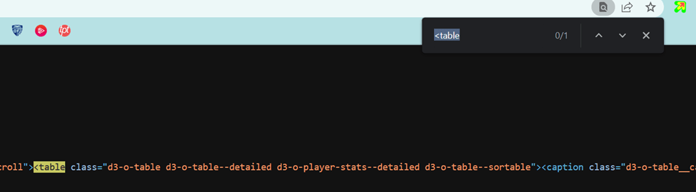
Since our target table is the first (and only) table on this page, our index will be 1.

Here is our initial formula:

=IMPORTHTML(“https://www.nfl.com/stats/player-stats/”, “table”, 1)

After we enter the formulate into A1, here is how the data appears:

Great, that was easy!  But we can use more Google Sheets features to improve this process.  I see several shortcomings with our current process:

1. We don’t need ALL of the columns from the source table.  I want to limit my data to only the fields I need to create my rankings.
2. I may want to specify some minimum criteria a player must meet before I import them (I have standards!).
3. I’d like a single, additional column that summarizes how well the player performed over the entire season.
4. Since I’m ranking these players, the best players should be at the top.

Let’s see how we can achieve these goals.

3.  Limit the Columns You Want to Import

There’s no point in cluttering up our spreadsheet with unnecessary data. Luckily, Google Sheets provides a way to only import the columns that we desire.

Looking at the columns on our target table, I’m only interested in a few of the columns.  

1.        Player (Column 1)

2.        Pass Yards (Column 2)

3.        TD (Column 7)

4.        INT (Column 8)

These columns are all the data that I need to help me rank these players for the upcoming season.

To limit the imported columns, we need to wrap our IMPORTHTML function in a query function.  The query function takes two parameters:

1. The data representing the range of cells on which to perform the query.
2. A query to perform, written in Google Visualization API Query Language.

For the data parameter, we’ll use the entire IMPORTHTML function that we’ve already built.  For the query, we’ll provide a query that targets the columns we want to include in our import.

=query(IMPORTHTML(“https://www.nfl.com/stats/player-stats/”, “table”, 1), “select Col1, Col2, Col7, Col8”)

Now our imported data looks like this, with no unnecessary columns!

So now we can successfully import the desired data set while also limiting the columns that will appear in our final sheets.  But there is still work to do.

4.  Filter Imported Rows Based on Custom Criteria

For my rankings, I only want to consider quarterbacks who threw for at least 3000 yards.  More generally, I want to filter the imported rows based on criteria in a specific column.

To create a filter, we’ll adjust our existing query function to include a WHERE clause.  Specifically, we’ll indicate that we only want to import rows where the value in Col2 is greater than or equal to 3000.

=query(IMPORTHTML(“https://www.nfl.com/stats/player-stats/”, “table”, 1), “select Col1, Col2, Col7, Col8 where Col2 >= 3000”)

Now, when we examine the result set, we can see that Lamar Jackson (the only player with fewer than 3000 yards passing) is omitted. Better luck next year!

Note: Lamar Jackson is a stud and we’d normally include him in our rankings.  This is theoretical, folks!

5.  Generate Fantasy Point Output Using a Calculated Field

We’ve successfully imported our raw quarterback stats, trimmed the columns to our liking, and filtered out some undesirable players.  That’s a great start toward creating our custom rankings.

But raw stats aren’t that helpful when it comes to fantasy sports.  What we really need to do is calculate the fantasy point output for each player.  That is a much better indicator of success.  

And sure, we could manually add another column, performing this calculation manually within our sheet.  But let’s instead streamline things by performing the calculation during the import process.

Developing a formula for fantasy points calculation

So what is the formula that we use to calculate fantasy point output for quarterbacks?

It turns out this formula will vary from league to league, based on your specific scoring configurations.  But for this tutorial, we’ll use a formula similar to the standard scoring system:

Fantasy Points = (Pass Yds / 25) + (TDs * 6) – (INTs * 2)

Adjusting the query to include the calculated field

To integrate the calculated field, we’ll adjust our existing query to include a calculated column. Specifically, we want to add our fantasy points calculation to the query parameter of the query function.

=query(IMPORTHTML(“https://www.nfl.com/stats/player-stats/”, “table”, 1), “select Col1, Col2, Col7, Col8, (Col2/25)+(Col7*6)-(Col8*2) where Col2 >= 3000”)

Now our spreadsheet contains the total fantasy output for each player (a much more helpful metric).

But that new column header looks really weird.  It’d be much cleaner if we could apply a custom label to the column (‘Fantasy Points’, for instance) l. It turns out this is possible, although the syntax is a bit odd.  

What we need to do is add more data to the end of our query:

1.        The keyword ‘label’

2.        Repeat the calculated field

3.        The desired column header as a string

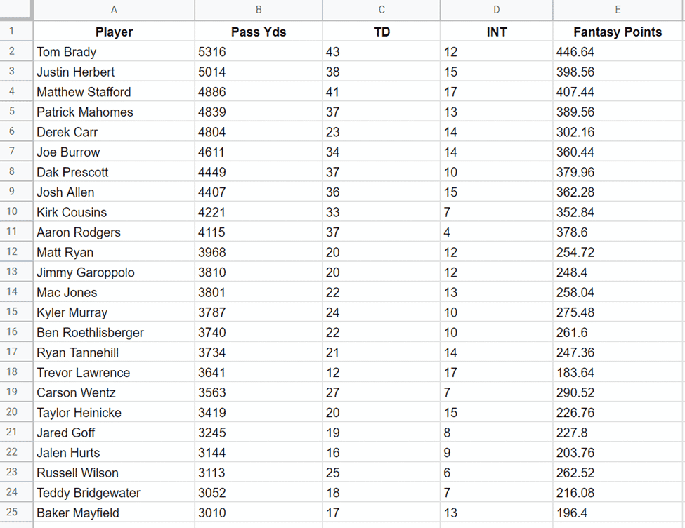
=query(IMPORTHTML(“https://www.nfl.com/stats/player-stats/”, “table”, 1), “select Col1, Col2, Col7, Col8, (Col2/25)+(Col7*6)-(Col8*2) where Col2 >= 3000 label (Col2/25)+(Col7*6)-(Col8*2) ‘Fantasy Points'”)

Now that’s more like it!

That Fantasy Points column is looking much better!  But I don’t think I need the decimal part of those numbers.  

To me, the decimal digits add unnecessary background noise. So let’s see if we can round up those numbers.

To accomplish this, we’ll apply a custom format to our query.  Specifically, we need to specify:

1.        The keyword ‘FORMAT’

2.        Repeat the calculated field

3.        The custom number format (“#” in our case)

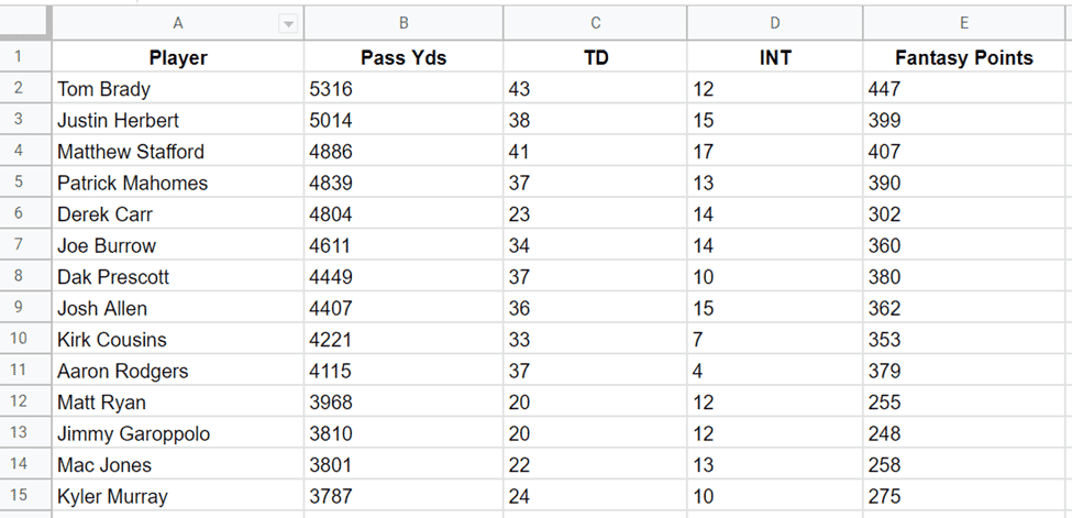
=query(IMPORTHTML(“https://www.nfl.com/stats/player-stats/”, “table”, 1), “select Col1, Col2, Col7, Col8, (Col2/25)+(Col7*6)-(Col8*2) where Col2 >= 3000 label (Col2/25)+(Col7*6)-(Col8*2) ‘Fantasy Points’ FORMAT (Col2/25)+(Col7*6)-(Col8*2) ‘#'”)

Now our table looks cleaner.

We’ve come a long way and have streamlined our data collection process. But we have one more step to complete this tutorial.

Since this exercise aims to create rankings for these players, it would be useful to sort them when we import the data.

Let’s work on that next.

6.  Order Rows Based on Calculated Column

We’ll again lean on our query to specify an initial row order for our data. We want to sort our rows by the calculated column (‘Fantasy Points’).  But we want to do this in descending order.

Sorting can be accomplished through the ORDER BY DESC clause. Again (and unfortunately), we’ll need to reference our full calculated field.  

NOTE: You cannot use the calculated field column header in the ORDER BY clause because in the SQL order of operations the alias isn’t applied until after the ORDER BY.

Here’s our final formula:

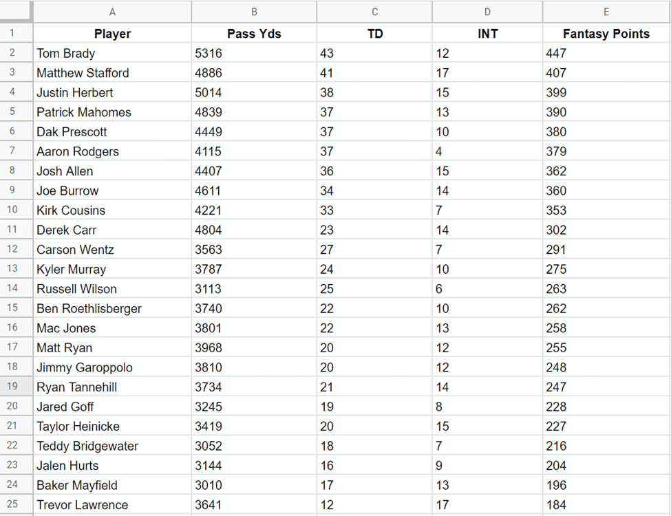
=query(IMPORTHTML(“https://www.nfl.com/stats/player-stats/”, “table”, 1), “select Col1, Col2, Col7, Col8, (Col2/25)+(Col7*6)-(Col8*2) where Col2 >= 3000 ORDER BY (Col2/25)+(Col7*6)-(Col8*2) DESC label (Col2/25)+(Col7*6)-(Col8*2) ‘Fantasy Points’ FORMAT (Col2/25)+(Col7*6)-(Col8*2) ‘#'”)

Our final data set is now ordered with the best players first (according to our league’s specific scoring rules).  

The Data Import Features of Google Sheets are Simple but Effective

Whether you’re a stats geek, student, or researcher, the versatility of the data import features in Google Sheets is a huge time-saver.  Using the functions detailed in this article, you now have the power to import, filter, sort, and further manipulate any data you can find on the Internet.  

And with over 6 billion web pages (and counting), it looks like you’re going to be very busy.

Atit Shah

Atit Shah is a digital marketing specialist. He is a true foodie who loves product marketing, e-commerce, traveling, and photography.